In addition to the static key figures for process and customer objects, which are displayed below the object symbols, the application also offers the option of automatically generating a time line below the objects.
This time line illustrates the individual statically determined processing times in the gradations value-adding (lower gradation) and non value-adding (upper gradation).
Figure 1 (of a simplified and thus not complete value stream for clarification) shows how the throughput times for value-adding processes (highlighted in green) are indicated accordingly at lower gradations of the time line and the non-value-adding throughput time of the Inventory objects at the upper gradation.
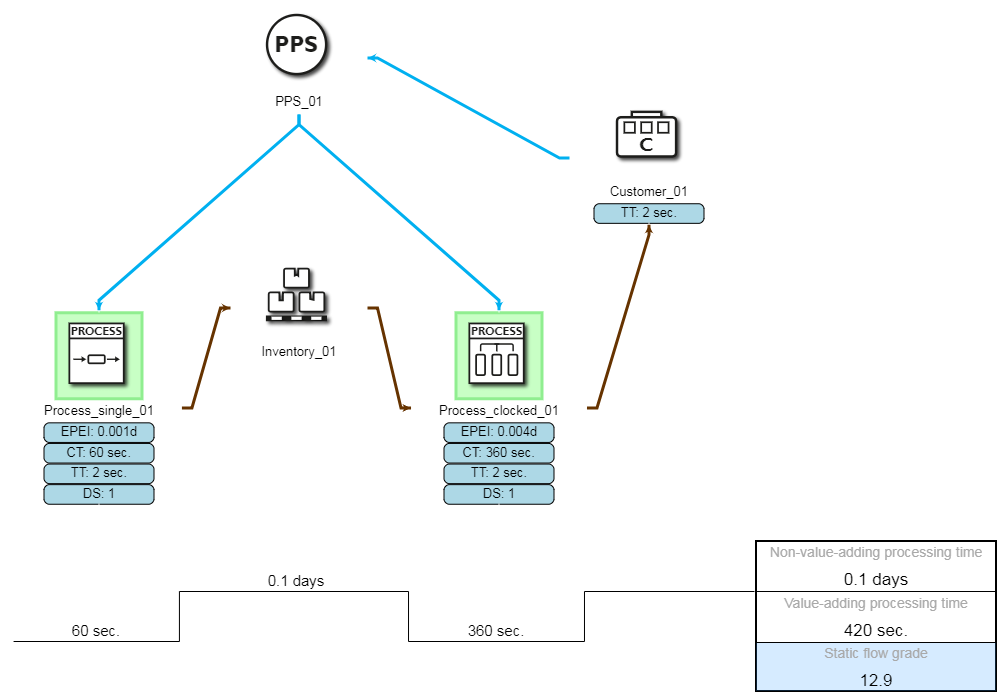
Figure 1 - Time line
In addition, Figure 1 shows how non-value-adding and value-adding times are cumulated and visualized at the right end of the time line.
Furthermore, in the box marked in blue below, the static flow rate is calculated as the quotient of the total throughput time (value-adding + non value-adding) and value-adding time (result values thus greater than 1).
Since the design of the time line is automatically oriented to the positions of the value stream objects and also automatically adapts to the attributes of the value stream objects, this central key figure of the value stream modeling can be read at any time.
Compared to Figure 1, Figure 2 shows an adjusted time line due to changed parameters with regard to cycle time and value added.
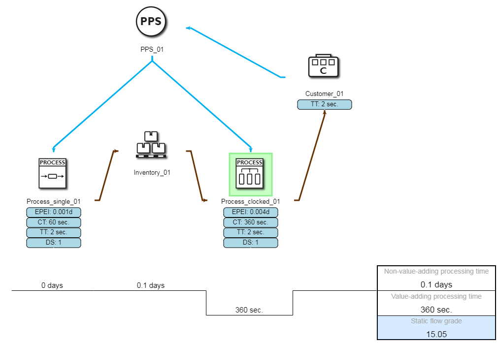
Figure 2 - Adjusted time line
The throughput times entered on the time line are calculated individually for each object type.
Thus, the throughput times of processes take into account the cycle time of products as well as the transfer quantity (TGT process formula).
In addition the capacity (Formel TGTProcess_clocked) is included for clocked processes and the throughput time (Formel TGTProcess_Lead) is included for lead processes.
For Inventory objects, the initial stock at product level (as the static admission value of the current stock) is extrapolated to a storage range of coverage in days using the average customer cycle (Formel TGTStorage).
Transport objects (FIFO, internal and external transport) are entered with the corresponding transport time.
For external transports, only the initial transport is used for the static throughput time calculation. (Formel TGTTransport).
By default, only one time line is generated below the modeling.
However, if the value stream modeling becomes more complex or even very branched (with parallel modeled objects), the application also offers the possibility to divide the modeling area into layers, which are used to create individual time lines.
Value stream objects whose symbol centers are then within the same modeling layer are assigned to a common time line. The number of layers is automatically determined based on the vertical positioning of the value stream modeling.
Thus, even with branched value streams (with parallel modeling), unambiguous time lines can be easily controlled according to the positioning of the objects and the assignment of the objects to individual time lines.
Figure 3 shows a value stream modeling with layers. For example, the second layer was used to exclude a parallel clocked machine from the time line calculation of the main line.
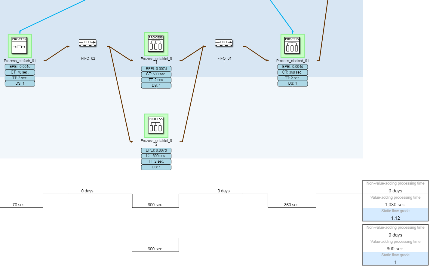
Figure 3 - Value stream modeling with layers
© SimPlan AG - Hanau District Court, Commercial Register (Part B) 6845 - info@simplan.de - www.simplan.de/en